Submodule interpolate

This submodule has several related features:

• A module polynomial with basic features to work with polynomials
• A module fitpack to performe interpolation/fitting using an expansion in B-splines
• A module csplines to work with cubic splines, represented as piecewise cubic polynomials

CubicSplines

CubicSplines gives a frame to interpolate data using Cubic Splines. It uses an internal representation as a list of piece-wise cubic polynomials. It has a functional interface and an Object oriented interface. Both modes of use are equivalent and they rely on the same implementation.

CubicSpline Object and methods

The use of the object oriented CubicSplines is very convenient, as it is illustrated in the following example

program cubic_splines_oo
  USE numfor, only: dp, linspace, save_array, str, m_pi
  USE numfor, only: cubicspline
  implicit none
  integer, parameter :: Ndim = 20, ndimnew = 4 * ndim
  type(CubicSpline) :: csp
  real(dp), dimension(Ndim) :: x, y
  real(dp), dimension(Ndimnew) :: xnew, ynew, yder
  real(dp), dimension(:), allocatable :: zeros
  character(len=:), allocatable :: header
  character(len=:), allocatable :: fname
 
  ! Create the data
  x = linspace(1.e-6_dp, 20._dp, ndim)
  y = sin(x)
  ! New grid
  xnew = linspace(1.e-6_dp, 19.99_dp, ndimnew)
  
  ! Create the CubicSpline
  ! Notice that we know exactly the second derivative
  csp = cubicspline(x, y, -y(1), -y(ndim))
  ! Apply the interpolation to the new grid
  ynew = csp%evaluate(xnew)
  
  ! save to file fname
  fname = "data/ex_interp_cspline1.dat"
  header = "x                sin(x)             evaluate"
  call save_array([xnew, sin(xnew), ynew], 3, fname=fname, fmt="f17.14", header=header)
  
  ! Given a CubicSpline object csp, evaluate the derivative
  yder = csp%derivative(xnew)
  
  ! save to file (stdout really)
  fname = "data/ex_interp_cspline2.dat"
  header = "x                cos(x)             derivative"
  call save_array([xnew, cos(xnew), yder], 3, fname=fname, fmt="f17.14", header=header)
 
  print "(A,f8.6)", "Value of the function at 1.5     = ", csp%evaluate(1.5_dp)
  print "(A,f8.6)", "Value of first derivative at 1.5 = ", csp%derivative(1.5_dp)
  print "(A,f8.6)", "Value of integral from 0 to 1.5  = ", csp%integrate(0._dp, 1.5_dp)
 
  zeros = csp%roots()
  header = "There are "//str(size(zeros))//π" roots. In units of :"
  call save_array(zeros / m_pi, 1, fmt='f13.10', header=header)
 
end program cubic_splines_oo

This outputs:

Value of the function at 1.5     = 0.993493
Value of first derivative at 1.5 = 0.066617
Value of integral from 0 to 1.5  = 0.927102
# There are 7 roots. In units of π:
-0.0000000025
 0.9999594164
 1.9999193799
 2.9998803876
 3.9998428449
 4.9998041860
 5.9995842765

and

$> cat data/ex_interp_cspline1.dat
 # x                sin(x)             evaluate
  0.00000100000000  0.00000100000000  0.00000100000000
  0.25303896202532  0.25034730035496  0.24863008190056
  0.50607692405063  0.48474965603025  0.48261414919792
  0.75911488607595  0.68827961288887  0.68730825131711
  1.01215284810127  0.84797489664940  0.84806743768314
 ...
 18.97784815189873  0.12794059510705  0.12747484922469
 19.23088611392405  0.37215544351995  0.36755693669675
 19.48392407594936  0.59266871498231  0.58580060371012
 19.73696203797468  0.77543651368883  0.77015926631456
 19.99000000000000  0.90881885124069  0.90858634055980
 
$> cat data/ex_interp_cspline2.dat
 # x                cos(x)             derivative
  0.00000100000000  0.99999999999950  0.99222241991253
  0.25303896202532  0.96815609754057  0.96328391891808
  0.50607692405063  0.87465294316006  0.87646892201067
  0.75911488607595  0.72544550069702  0.73177742919030
  1.01215284810127  0.53003638993227  0.52920944045695
 ...
 18.97784815189873  0.99178183292681  0.97608188013021
 19.23088611392405  0.92817041854310  0.91358086898952
 19.48392407594936  0.80544633234078  0.80347204495850
 19.73696203797468  0.63142554053358  0.64575540803714
 19.99000000000000  0.41719095823083  0.44043095822545

Note that in order to get the interpolated values only three lines are relevant:

• line 3: where the object is declared.
• line 20: where the interpolation to the data is determined.
• line 22: where the interpolated values are obtained.

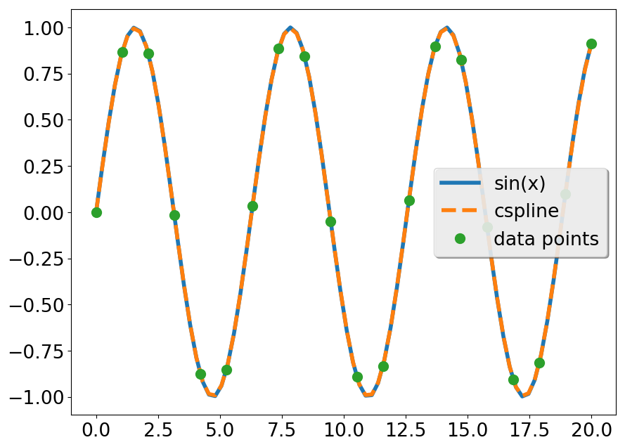
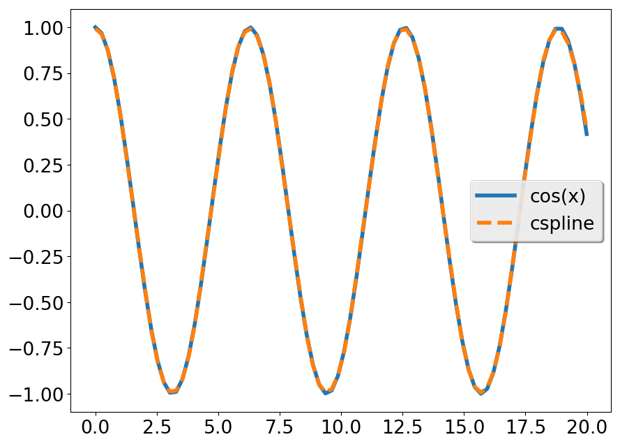
The evaluation of the data in the new points results in:

while the derivative gives

Note

that both interpolations are particularly good at both ends because we gave good values for the second derivative.

CubicSpline Functions and subroutines

Interpolation using cubic splines may be accomplished in a very similar manner using the functional interface to CubicSplines. Its use is very similar to the object oriented aproach, as shown in the translation of the above example to this interface

program cubic_splines_fp
  USE numfor, only: dp, linspace, save_array
  USE numfor, only: cubicspline, csplrep, csplev, csplevder, csplint
  implicit none
  integer, parameter :: Ndim = 20, ndimnew = 4 * ndim
  type(CubicSpline) :: csp
  real(dp), dimension(Ndim) :: x, y
  real(dp), dimension(Ndimnew) :: xnew, ynew, yder
  character(len=:), allocatable :: header
  character(len=:), allocatable :: fname
 
  ! Create the data
  x = linspace(1.e-6_dp, 20._dp, ndim)
  y = sin(x)
  ! New grid
  xnew = linspace(1.e-6_dp, 19.99_dp, ndimnew)
  
  ! Create the CubicSpline
  ! Notice that we know exactly the second derivative
  call csplrep(x, y, -y(1), -y(ndim), csp)
  ! Apply the interpolation to the new grid
  ynew = csplev(xnew, csp)
  
  ! save to file
  fname = "data/ex_interp_cspline3.dat"
  header = "x                sin(x)             evaluate"
  call save_array([xnew, sin(xnew), ynew], 3, fname=fname, fmt="f17.14", header=header)
  
  ! Given a CubicSpline object csp evaluate the derivative
  yder = csplevder(xnew, csp)
  
  ! save to file
  fname = "data/ex_interp_cspline4.dat"
  header = "x                cos(x)             derivative"
  call save_array([xnew, cos(xnew), yder], 3, fname=fname, fmt="f17.14", header=header)
 
  print "(A,f8.6)", "Value of the function at 1.5     = ", csplev(1.5_dp, csp)
  print "(A,f8.6)", "Value of first derivative at 1.5 = ", csplevder(1.5_dp, csp)
  print "(A,f8.6)", "Value of integral from 0 to 1.5  = ", csplint(0._dp, 1.5_dp, csp)
end program cubic_splines_fp

Fitpack

This module allows to either fit or interpolate data using an expansion in B-splinebasis of order . The implementation is based in the FITPACK set of routines by P. Diercxx.

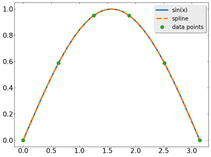
Use of splrep() with splev()

The first example illustrates how to use B-Splines to interpolate a function y=f(x) from a few data points:

program ex_splprep
  USE numfor, only: dp, zero, m_pi, str, linspace, save_array
  USE numfor, only: univspline, splrep, splev
  implicit none
 
  integer, parameter :: N = 6
  integer, parameter :: Nnew = 29
  real(dp), dimension(N) :: x
  real(dp), dimension(N) :: y
  real(dp), dimension(Nnew) :: xnew
  real(dp), dimension(Nnew) :: ynew
  character(len=:), allocatable :: header
  character(len=:), allocatable :: fname
 
  real(dp) :: s
  type(UnivSpline) :: tck
 
  ! Create data
  s = 0._dp
  x = linspace(zero, m_pi, n)
  y = sin(x)
  xnew = linspace(zero, m_pi, nnew)
  
  ! After setting data in x
  ! interpolate: (step one) Create interpolation and parameters u
  call splrep(x, y, tck=tck, s=s)
  ! interpolate: (step two) Apply to points u
  call splev(xnew, tck, ynew)
  
  ! save to file
  fname = "data/ex_interp_splrep1.dat"
  header = "x                   y"
  call save_array([xnew, ynew], 2, fname=fname, fmt="f17.14", header=header)
end program ex_splprep

Prints:

$> cat data/ex_interp_splrep1.dat
 # x                   y
 0.00000000000000  0.00000000000000
 0.11219973762821  0.11401345780438
 0.22439947525641  0.22522911715938
 0.33659921288462  0.33269883705930
 0.44879895051283  0.43547447649845
  ...
 2.69279370307697  0.43547447649845
 2.80499344070517  0.33269883705930
 2.91719317833338  0.22522911715938
 3.02939291596159  0.11401345780438
 3.14159265358979  0.00000000000000

Notice that we force interpolation by using s=0,

Use of splprep() with splev()

This second example illustrates how to use B-Splines for a parametric curve in the plane.

 
program ex_splprep
  USE numfor, only: dp, zero, m_pi, str, linspace, save_array
  USE numfor, only: univspline, splprep, splev
  implicit none
 
  real(dp), dimension(:), allocatable :: r, phi, u
  real(dp), dimension(:, :), allocatable :: x, new_points
  type(UnivSpline) :: tck
  character(len=:), allocatable :: header
  character(len=:), allocatable :: fname
 
  integer :: Nd = 40          ! Number of points
  real(dp) :: s = 0._dp
 
  allocate (r(nd), u(nd), phi(nd))
  allocate (x(2, nd), new_points(2, nd))
 
  ! Create data
  phi = linspace(zero, 2 * m_pi, nd)
  r = 0.5_dp + cos(phi)        ! polar coords
  x(1, :) = r * cos(phi)      ! convert to cartesian
  x(2, :) = r * sin(phi)      ! convert to cartesian
  
  ! After setting data in x
  ! interpolate: (step one) Create interpolation and parameters u
  call splprep(x, u, tck, s=s)
  ! interpolate: (step two) Apply to points u
  call splev(u, tck, new_points)
  
  ! save to file
  fname = "data/ex_interp_splprep1.dat"
  header = "u                    x                   y"
  call save_array([u, new_points(1, :), new_points(2, :)], 3, fname=fname, fmt="f17.14", header=header)
end program ex_splprep
 

Prints:

$> cat data/ex_interp_splprep1.dat
 # u                    x                   y
 0.00000000000000  1.50000000000000  0.00000000000000
 0.03616230734577  1.46779335229253  0.23853963732962
 0.07211603380768  1.37398960267532  0.45870512901973
 0.10765440708122  1.22676038619218  0.64385351896871
 0.14257428865429  1.03883011365998  0.78063018793468
 ....
 0.85742571134571  1.03883011365998 -0.78063018793468
 0.89234559291878  1.22676038619218 -0.64385351896871
 0.92788396619232  1.37398960267532 -0.45870512901973
 0.96383769265423  1.46779335229253 -0.23853963732962
 1.00000000000000  1.50000000000000 -0.00000000000000 

Notice that:

1. We force interpolation by using s=0,
2. The parameterization array u is generated automatically.